
Two Problems
Someone has given you a new shiny project to do, so you’ve got a problem that needs a solution. Thing is now you have two problems, the easy one is probably the shiny project, the harder one is managing the stakeholders.
To avoid poor project outcomes some stakeholders (like managers) will just want information, some are providing resources to the project and some have to be managed to prevent them derailing or threatening the project’s success.
First Steps in Stakeholder Analysis
As with anything in project management the first step is always to make a list that captures something of the problem you’re facing and from that we can pull out some germ of truth to help us figure out what to do next.
So in your list gather:
- The stakeholder’s name, email, handle, etc.
- The stakeholder’s role or relationship to the project, and any groups you can identify
- The stakeholder’s project power vs project interest (optional)
We’ll explore these topics in a bit more depth now.
Roles
When ordinary people become stakeholders in a project some of their expectations as stakeholders differ on account of the different roles that the stakeholder plays. For example, the managing director of your firm will have a different point of view on the project to the lead developer, which will be different again than the point of view of the firm’s clients.
Some key roles to look out for in your project are:
- Sponsor – the person who wants this project and whose word is final on the project. This person can clear the path of potential issues around and above the project (if necessary). Ideally it’s just one person, if it’s more than one try to make it one because it removes a potential political hurdle when dual sponsors have different views.
- Subject Matter Experts (SMEs) – these are easy to spot, they’re the people that you can consult on more technical aspects or specifics. They may or may not be people that contribute directly to the project, but having an SME agree with you (or you agreeing with them!) is never a bad way to be.
- Project Managers – you might think you’re the project manager, but often there are other people on the periphery who will exert control over the project without explicitly being given authority to do so. It’s good to identify the people that might do this, if only to communicate what the lines of responsibility actually are.
- Project Team – the workers, this might include you but generally it’s anyone who will work on the project in whatever capacity. If you have lead engineers or support staff it’s useful to identify this too (so that when you share this information other people can use it like a directory).
- Externals – so if you have external stakeholders to your organisation then the chances are their opinion is quite important. This is likely because they’re clients or they will be beneficiaries or affected by the project in some way. They will probably not contribute much to the project but you need to understand them. If you have more than one type of external stakeholder, record that as well.
Power vs Interest (optional)
There are many things you can do with stakeholder analysis. They’re all designed to give you insight into what people might expect. Power vs interest is a very common and reasonably useful way, but there are plenty of others, each with their own strengths and benefits.
To be honest there’s no absolute need for this but you might do it for two reasons:
- It’s sometimes quite revealing to formulate opinions on people’s expectations through this lens.
- It can be quite fun!
Before you make the list though, be careful to consider who might see your list. Even though you may try to be truthful/accurate you may find the people you have captured information on disagree with your categorisations. Which can be both embarrassing and frustrating, so consider whether you will make two lists. One to communicate and share with the other stakeholders, and one that is just for you to understand their motivations.
If you do decide to try it, it’s very straight forward. For each of your stakeholders mark them out of 10 in terms of their power/influence on this project (0=no power or influence, 9=very powerful/influential) and then mark them again for their interest (0=no interest, 9=very interested).
Then plot them on a scatter chart, where they appear on that diagram will influence how you communicate with them.
- Bottom left – no power/no interest – you don’t want too many people in this quadrant if you do you might have a problem delivering the project.
- Top left – lots of power/no interest – keep these people up-to-date they have the ability to derail your efforts.
- Bottom right – no power/lots of interest – hopefully the junior members of your project team is in here somewhere.
- Top right – lots of power/lots of interest – hopefully your sponsor, PM and more senior project team members are in here.
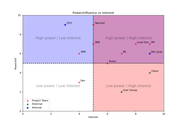
These things are very subjective, so when you plot it first time it probably won’t feel quite right. You might have scored some of the people on different aspects of power/interest (since there are many). So tweak it a bit until it feels like you can justify the diagram as a whole.
Putting it all together
You’ve got your list, you’ve plotted your scatter diagram what now? Well if you’re lazy like me you might leave it there. You’ve done the analysis, you know more now than you did at the start, but some more useful things you could do with your stakeholder analysis are:
- Communicate On It – I’ve hinted at this already, but it’s very helpful for everyone to know what their role is on a project. It helps set their expectations from you and your expectations of them. I’d personally just share the version with just names and roles in it at the start of the project. If questions arise at this stage it’s good to get them out in the open.
- Plan From It – a lot of the people in your stakeholder analysis are likely to be key resources in your project. Having them, their diaries and their availability easily accessible in your project folder makes everything a bit simpler.
- Reorganise the Team – if after doing the power vs interest analysis you decide that your team isn’t balanced, and you have scope to do it, use the analysis to reorganise the team or make some substitutions. To be honest though I’ve rarely had this luxury.
- Communicate With It – a lot of successful project management is about communication. If you understand the stakeholders then you can tailor the communications to suit the stakeholders. For example the sponsor is employing you to handle the details, so high level progress and issues will probably be fine for them – but it depends on their level of interest. The SMEs and externals probably just like to know high level progress but you might phrase it differently for each audience. Finally, the project team probably want short term detailed plans. So, come up with a small suite of reports and decide who gets what report and use your analysis as a guide to the distribution and content.


 And this is the bit that makes me a bit sad inside. This is what OO was really meant for. I used to have arguments with business-analysts about the right object model to use and whether a method should exist in a base-class or a derived-class. But now it doesn’t seem like anyone, including me, really cares. It’s just that somewhere along the line it became a little irrelevant. Don’t get me wrong, I work with objects all the time. But they’re not really objects that were sold to me.